Goodbye %>%, Hello := (Using R data.table to speed up my data science)

This is a little story about how I learned to stop worrying and love data.table, a great (and in my opinion underrated) package for doing data science in R.

I have used R since 2011, and initially learned to work with data using mostly base R code. In about 2013 I started using the plyr package, which later morphed into dplyr and, along with some other packages, was dubbed the “tidyverse.” I have long admired the tidyverse’s design philosophy. It’s really helped me speed up writing data analysis and processing scripts interactively. But there are some negatives of tidyverse. It’s not very stable: code from a few years ago often breaks if you are keeping your package and R versions up to date. More importantly, it doesn’t care that much about code being fast or lean in terms of memory use. Enter data.table.

Why did I learn it?

Both data.table and tidyverse are really well-designed but have different goals. The main goal of data.table, a package developed by Matt Dowle and Arun Srinivasan, is to quickly and efficiently manipulate huge data frames with millions of rows. Functions in data.table are optimized to use as little memory as possible by avoiding making unnecessary temporary copies of data frames. This results in code that is more efficient in both time and memory use. Another advantage is that data.table is much more stable than tidyverse, even though it has actually been around for longer (since 2008), and is constantly being updated. The old data.table code still works. Another nice feature is that it has no dependencies — contrast that with the large number of back-end packages now required to run the tidyverse.

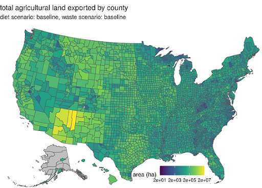
For my food waste research I had a “big data” problem. My data includes pairwise flows of 10 different goods between all pairs of the ~3100 counties in the United States, replicated over 20 different scenarios. That’s 20 * 3100^2 * 10 which ends up being a huge data frame. Just doing basic operations in tidyverse such as pivot(), summarize(), and mutate() was taking a day, even if I ran the code split up across a lot of cores in parallel on the Slurm cluster. Because I was still trying to work out some kinks in the analysis, it was annoying to have to run code for a day every time I wanted to check if the full analysis worked. That’s why I thought it would be nice to learn data.table. It had been on the back burner for a long time but this time I actually decided to sit down and learn it.

Image

Some examples

If you’ve used tidyverse you have certainly seen the %>% (pipe) operator. The pipe allows you to chain many data-manipulation commands into one statement without having(to(nest(functions(like(this))))).

data.table also has a signature operator, :=. This is a special assignment operator that lets you create new data frame columns in-place without having to reassign the entire data.table to a new object. This saves time and memory.

For example, in tidyverse you could write

mydata <- mydata %>%
  mutate(new_column = column1^2 + column2)

The equivalent in data.table would be

mydata[, new_column := column1^2 + column2]

You don’t need to assign anything — mydata is modified in place.

You can also chain commands in data.table using brackets, so you can write statements in a similar way to tidyverse if that’s your style.

For example, this in tidyverse:

mydata %>%
  mutate(log_population = log(population)) %>%
  filter(year > 1990) %>%
  group_by(country, city) %>%
  summarize(log_pop_density = log_population/area)

is this in data.table:

mydata[,
  log_population := log(population)][
  year > 1990][
  .(log_pop_density = log_population/area), by = .(country, city)]

How did I learn it?

I went through the vignettes on data.table’s homepage, which are a very nice tutorial that I would recommend to beginners who are otherwise familiar with R.

In the end it was helpful that I first learned data manipulation in base R, before tidyverse had taken over the world. Because data.table’s syntax is a little closer to base R syntax than tidyverse’s, some things were more familiar to me than if I had only learned tidyverse ways of doing things. That’s a little like a native English speaker learning German, where you occasionally recognize a cognate or bit of grammar that resembles “old-fashioned” English.

Hybrid solution

In the end, I rewrote my food waste data processing code using mostly data.table syntax with some of the map() family of functions from the purrr package (Jenny Bryan’s excellent tidyverse list manipulation package) mixed in. I also found a few custom functions through the art of Googling that allowed me to mimic some tidyverse behavior, in particular grouping a data.table and making a list column in each group. data.table supports list-columns in data frames — in fact, it has had that useful feature since the beginning, which was only later adopted by tidyverse packages. Maybe my solution isn’t the optimal data.table solution but it helped me translate my code from tidyverse to data.table without having to completely rethink how it’s done.

There are other options that allow hybrid solutions where code written in tidyverse language can run with data.table’s performance, or even packages like dbplyr that let you use SQL databases while writing your code in tidyverse language (data.table is also based on SQL). This would be nice if you really like the %>% better than the :=. But data.table also has some appealing syntax — I am enjoying writing code in data.table!

Take-home message

I am happy with the performance benefit I got from learning data.table (roughly a 3x speedup), it was a fun learning experience, and it’s always nice to learn a new language, or new syntax within a language. Just like learning a new foreign language, it helps your mind get out of set ways of thinking and frees you to come up with more creative solutions even in the language you already know. Of course it also fits with my quest to make my code more efficient and thereby get the same outcome while consuming less energy!